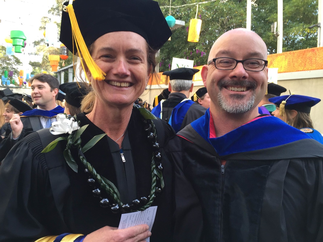
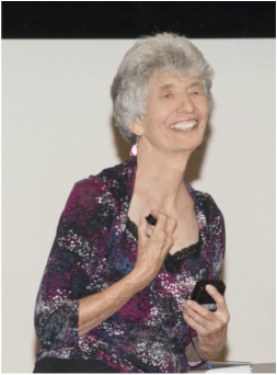
The College of Natural Resources held their 2015 commencement last night. Lisa finished her dissertation last summer and has been teaching in Monterrey for the past year but she came to walk and get hooded. Congratulations Lisa!
| O'Grady Lab |
|
|
The College of Natural Resources held their 2015 commencement last night. Lisa finished her dissertation last summer and has been teaching in Monterrey for the past year but she came to walk and get hooded. Congratulations Lisa!
1 Comment
Mike Peterson just wrote up a short review of our lab's Hawaiian biodiversity projects for the Berkeley Science Review. Thanks Mike!!
Great news! Graduate student Natalie Stauffer has been awarded several fellowships in the past two weeks. She received a Resh Award for her research and an O&E summer student fellowship that will pay stipend for summer 2015. She was also just selected for a Berkeley Connect position for the 2015-2016 academic year. Excellent work Natalie!
Nina Pak has been admitted into the graduate program in the Department of Environmental Sciences, Policy and Management! While she won't be changing labs, everyone is excited to have her stay in the lab as a PhD student.
She was also just awarded a summer research fellowship with the National Taiwan University. She'll spend the summer working in a research lab in Taiwan (and maybe collecting canacids and ephydrids) before coming back to Berkeley to start grad school in the fall. Congratulations!!
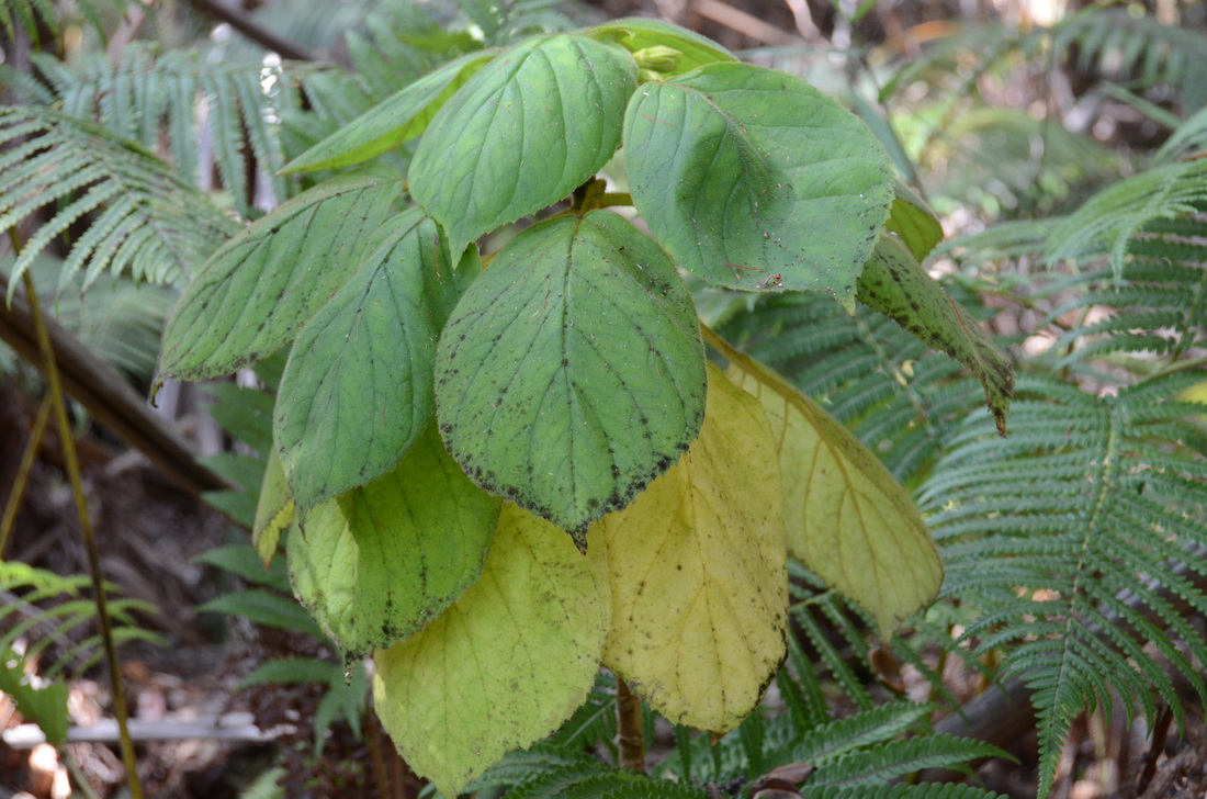
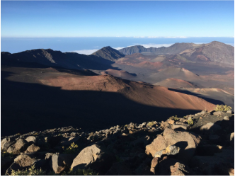
  We went to the Big Island and Maui to collect material for a couple different projects. My primary goal was to obtain samples of spoon tarsus species for our Dimensions in Biodiversity grant. I also wanted to obtain some more material from Scaptomyza cyrtandrae and a new species in that group from Maui that I'm describing with former student Jessica Craft. Finally, Nina and I were looking for canacids to expand the sampling within her phylogeny of Hawaiian Canacidae. It was a very successful trip and we got everything we needed for all the projects.  Kipuka along Puu Oo Trail. Mauna Kea is in the background. Click photo to see full panoramic view.
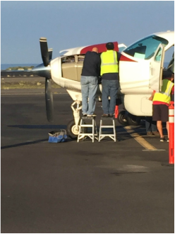
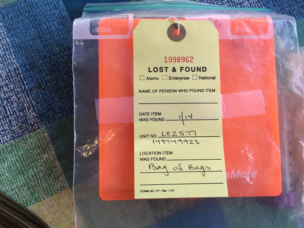
We flew over to Maui for a short two day trip. The flight over was very smooth but there were some problems with the plane before we took off. We spent the first day collecting canacids and ephydrids along the Hana Highway. The second day was spent in the Waikamoi Forest Reserve. East Maui Irrigation gave us access and helped out with logistics. We ended up leaving some of our collections in the rental car but the folks at National sent them to us in Hilo via Air Cargo.
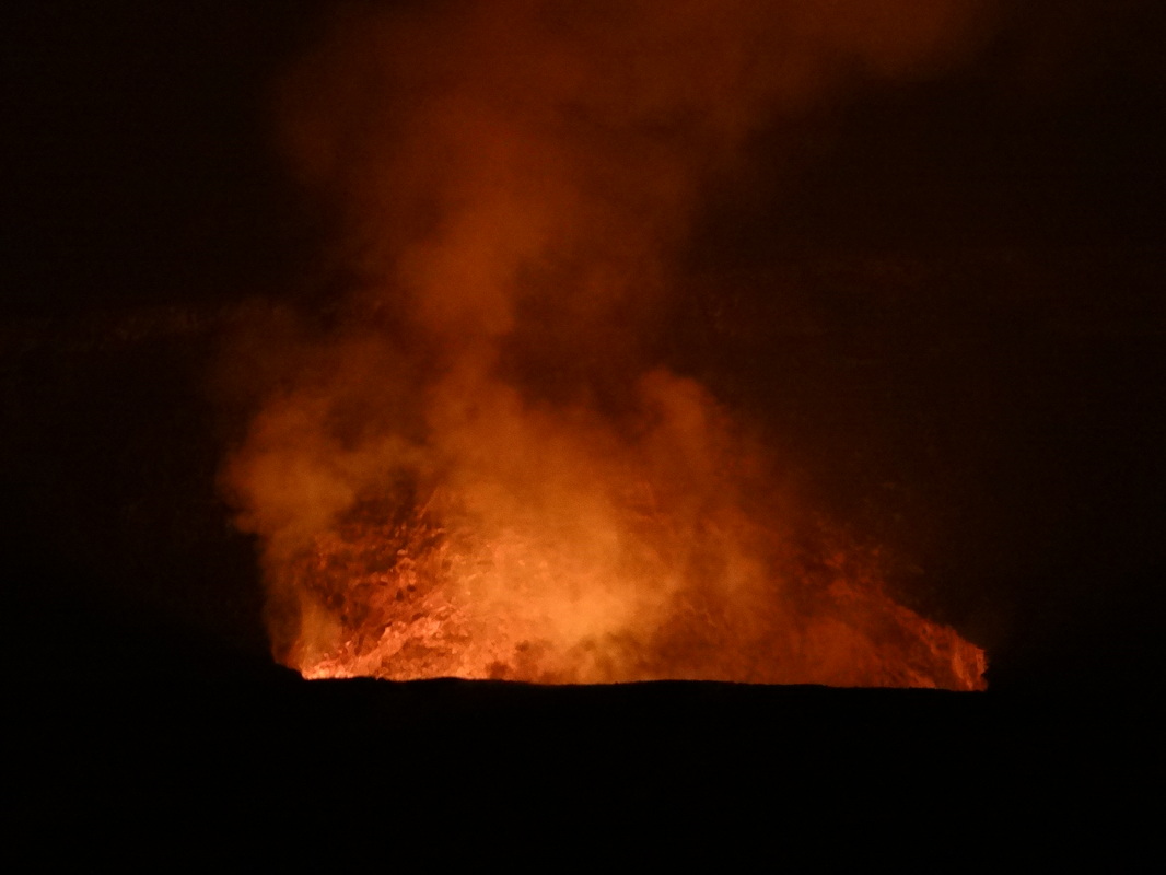
In addition to all the hard work we also go to do some touristy stuff. The Halemaumau Crater was very impressive at night and Haleakala Crater is always amazing.
Studying biodiversity is inherently interesting - at least to me - but too much biodiversity can bog you down when it comes time to reconstruct a phylogeny or produce a taxonomic revision. You simply cannot collect, identify, and sequence 1000 species in any reasonable amount of time (e.g., over the course of a 3-year NSF grant or in the 7 pre-tenure years at most academic institutions). Revisionary systematics, by its very nature, tends to produce large, tome-like publications, some of which take years to compile, refine and format. This creates an entirely different sort of pressure for researchers working within an academic "publish or perish" context. Not only do you need solid, preferably published, preliminary data to serve as a proof of concept for grant proposals, if you only publish one or two large papers per year you may not meet the standards for tenure at most institutions. To compound matters, taxonomic revisions tend to be the work of one or two authors working in almost total isolation. Long author lines with dozens of collaborators are virtually unknown in taxonomy. There is little culture of collaboration in modern taxonomy and this must change if the speed and breadth of species descriptions is to increase in the coming years.
The genomics revolution, with well-designed pipelines capable of generating and analyzing amazing amounts of data, has revolutionized how we think about data of all sorts. Big data initiatives, such as UC Berkeley's BIDS Program, are now common in science and pipelines for cybertaxonomy (e.g., Miller et al. 2012) are now helping ease the bottleneck surrounding revisionary work. Several authors have proposed a cultural change with how taxonomic publications are created and in how intellectual credit is awarded within academia. Several have promoted the notion of "quantum contributions" as a potential mechanism for increasing the rate of biodiversity discovery (Maddison et al. 2012; Riedel et al. 2013). A number of web-based journals (Zootaxa, Zookeys, Biodiversity Data Journal) and data hosting sites (Figshare) are making it possible to provide easy, open access to taxonomic data while attributing the contributions of various authors. While I'm not prepared to entirely switch to a quantum approach to all my publications, I do feel strongly that open access to all research output is critical in increasing the rate of biodiversity discovery. I have begun to use Figshare in three distinct ways. First, I've posted bits of published data (figures, data matrices, etc.) in an effort to make older information that might be behind paywalls more generally available. Second, I've posted projects that were conducted in my lab and are likely useful to someone but never quite got published on their own. Most notable among these are a study on the population genetics of Drosophila suzukii, an invasive drosophilid that has become a pest in cane fruits and other crops (Ort and O'Grady 2013), and a coevolutionary study of some Neotropical batflies (Diptera: Streblidae) and their hosts (Bennett et al. 2014). Finally, when someone requests unpublished information from me, rather than simply emailing it to them, I have been posting it so it is more widely available. Two recent examples of this are my collection records (Ku and O'Grady 2013) and a large donation of Bill Heed's repleta group stocks deposited in the AMNH's Monell Cryo Collection (O'Grady 2014). I plan on continuing to post these types of contributions to Figshare and will be monitoring how much use they actually get. It's been about a year since I started doing this and I have over 800 views - but no citations yet. One of the main goals of my sabbatical was to write, write, write. I needed to finish up a number of papers that had been on the back burner for way too long. I also wanted to start a couple larger projects. While I didn't get everything done that I wanted to, I was able to make strong progress on all my writing projects. I also managed to add another paper, coauthored with my host, Noah Whiteman, and his lab. This turned out to be a nice project that allowed us to summarize some of the microbial work that we have both been doing in our labs. This paper has just come out online in Frontiers in Microbiology's special Symbioses issue. Here's a link to the paper.
Kari's latest paper on Hawaiian Diptera is out! This one is a phylogeny of the endemic Hawaiian Campsicnemus (Diptera: Dolichopodidae), with some very interesting analyses on the biogeography and ecological adaptations in the group. Our coauthors were Neal Evenhuis at the Bishop Museum and Pavla Bartosova-Sojkova, a former visiting scholar in the lab. We have one more paper on Hawaiian dolis in the works and are excited to publish on this very cool radiation of about 350 endemic Hawaiian species.
I posted earlier this year about wanting to publish a series of small papers on the distribution and identification of several lineages of Hawaiian flies. I also wanted to use the series to publish some species names from the smaller groups or the clades where a full revision isn't tractable. The first paper was on the Asteiidae and it came out in February. The second in the series was on the genus Scatella (Ephydridae) and was published in August. My coauthors Neal Evenhuis and Keith Arakaki are both researchers at the BP Bishop Museum. We owe a huge thanks to Torsten Dikow for helping with the database of the Smithsonian Material. You can read the paper here.
My next paper will be on the endemic Hawaiian Canacidae and will include the description of a new species in the genus Procanace. |
PatrickProfessor Archives
April 2018
Categories
All
|
 RSS Feed